The NEAT Algorithm: Evolving Neural Networks

Preface: On Searching the Archives
Unless you live in a cave you’re probably well aware that Neural Networks have been experiencing something of a renaissance of late. Abandoned as interesting-but-a-dead-end not too long ago, the relentless march of Moore’s Law means now we have the computing power required to exploit these statistical automata. As marketing departments jump up and down with delight at being given a means of generating seemingly endless streams of hyperbole, it’s worth asking what other ideas are out there that have yet to have their day?
What Else Is Out There?
With almost the entire corpus of computer science knowledge encoded in LLMs, why can’t we just ask a Large Language Model (LLM) for a list of good candidates? Well, I tried that, the results are… suboptimal… and while the response from proponents of Generative AI may be "You’re just not using it right" I say to them (and you), it’s much more fun to look through the literature yourself and train the neural network between your ears to do the work (after all it has many more connections).
I don’t propose we should scour the literature for the next paradigm shift - the next DynaBook or Xanadu. I wouldn’t ignore it if I were to stumble across it, of course, but there is a huge amount of utility in looking for the clever techniques which have solved difficult problems on a less grand scale. You never know what you’ll find, and you never know what will prove useful.
Doesn’t that sound more fun than spending hours crafting just the right prompt?
Neuro-Evolution of Augmenting Topologies (NEAT)
In this post I’d like to share something that’s perhaps not exactly a forgotten relic, but certainly something that’s not very well known - the NEAT algorithm.
I’ll cover:
-
What the NEAT algorithm does.
-
An in-depth explanation of how it works.
-
Some examples of implementations of NEAT so you can get hands-on with it.
-
Some extensions/adaptations to the NEAT that improve its ability to solve different classes of problems.
What Does NEAT Do?
Imagine pointing a software program that knows nothing, about anything, at Super Mario World. You walk away to make something to eat and when you come back it’s playing the game so skillfully that you assume a human must be playing remotely.
This is what NEAT does, it is an algorithm which creates a neural network that solves whatever problem you define.
To be more precise, NEAT is a Genetic Algorithm which evolves the least complex network topology capable of approximating a target function. The neural networks NEAT outputs are capable of displaying extremely complex behaviours.
Rather than starting with a fixed topology created by a human, NEAT starts with a simple neural network topology (for instance, each input node connected to a single output node) and a fitness function and iteratively adds structure to the topology (i.e. adding a new node or a new connection between existing nodes, perturbing the weights of nodes, changing the activation function of a node, etc., etc.) until the output of the network satisfies the error threshold of the fitness function.
And if you don’t believe me about the Mario thing, here’s a video.
How Does NEAT Do It?
The original NEAT paper, Efficient Reinforcement Learning through Evolving Neural Network Topologies, published in 2002, was co-authored by Kenneth Stanley and Risko Miikkulainen. In this paper the authors outline the details of the techniques, unique to the NEAT algorithm, which allow an evolutionary approach to not only efficiently encode a neural network topology as a set of virtual genes but also to allow for the preservation of structural innovation necessary to avoid evolution stalling in local minima.
Before we dig in to the specifics of NEAT, here’s some background on Genetic Algorithms in general. If you already know about this class of algorithms feel free to skip down to Encoding a Neural Network Topology
Genetic Algorithms
Genetic Algorithms (GAs) are a type of metaheuristic, meaning they are a means of finding a 'good enough' solution to a problem so complex it would be inefficient to find the optimal solution. Metaheuristics are often employed when trying to find feasible solutions to NP-Hard problems such as Travelling Salesman or Job Shop Scheduling. They are sometimes referred to as Partial Search solutions, indicating that they’re focussed on finding and evaluating a subset of the possible solutions, rather than all possible solutions.
Think about it this way: do you want to find a feasible solution which is good enough in a minute or two, or do you want to wait, possibly until the heat death of the universe, for the best possible solution?
Evolving Solutions
GAs are a biologically-inspired class of algorithm, perhaps the ultimate biologically-inspired class of algorithm in that, unlike algorithms that mimic the behaviour of flocking/schooling/swarming animals such as birds or social insects, they mimic the evolution of living things themselves.
I’m sure you’re familiar with the process of evolution (even if you don’t believe in it - after all it’s just a theory, right?), but let’s review the process in a way that will make it easier to see the comparison between the process and NEAT’s implementation of it.
Requirements
Implementing a Genetic Algorithm requires two things:
-
An Encoding Scheme
-
A Fitness Function
Encoding
In the same way that the genetic information of living things is encoded in a Genome, we need to encode the problem we wish to evolve a solution for in a way a software program can understand. Generally, an array of numbers is sufficient. When we try and encode a neural network topology, however, that’s more of a challenge - not the encoding of the information about the nodes itself, it’s not too hard to come up with a few viable options for this - but how do we produce an encoding which lets us easily compare the difference between one node and another?
Think about it this way, consider the two network topologies in Figure 2. How can we select genes from one parent and genes from another which will be guaranteed to produce a viable child network? How do we know that all the nodes in the resulting child will be connected to other nodes? That all input nodes will be connected to either an output node or a hidden node? And, conversely, that all output nodes will have an incoming connection?

Fitness
Once you’ve found a way to encode your problem you need a means of evaluating the result of the network. With optimisation problems we use an Objective Function which tells us whether a candidate solution meets all the constraints of the problem definition. With Genetic Algorithms we use a Fitness Function.
The purpose of Fitness is to have some means of comparing one candidate solution with another, to see which one is closer to the optimal result.
The Fitness Function takes a candidate solution, extracts the values encoded in the candidate solution, assesses the result of applying those values to our problem and outputs a score which represents the 'Fitness' of that solution.
The type of the Fitness score (the type of object returned by the fitness function) can be anything as long as we have a way of comparing instances of those types with each other (so, numbers are pretty useful). We can compare the current candidate with the previous best solution and, if it’s better, we have a new champion.
Selection of the Fittest
Just as in nature, our Genetic Algorithm follows a fairly simple process (there are variations on this process, but this is the basic idea):
-
Start with an
Initial PopulationofGenomes -
Calculate the
Fitnessof eachGenomein thePopulation -
Select the fittest members of the
Population -
Pair the fittest members and create offspring by taking some genes from one parent and some genes from the other
-
Randomly mutate some of the offspring
Genomes -
Place all the offspring in a new
Population -
Calculate the fitness of the members of the new
Population -
Repeat from Step 3 using the new
Population
Each time we create a new Population we have a new Generation of Genomes with which we are gradually exploring the solution space to our problem. Theoretically, selecting the fittest members (those closest to our target objective) for breeding the offspring should have a higher likelihood of being closer to the objective than their parents in the previous Generation.
By optionally mutating the genes in some of the offspring we add some perturbation to the process, helping to prevent the process from getting trapped in local minima. Again, this mimics biological evolution in that these mutations can either increase or decrease the fitness of the individual but they are useful in helping a species escape a local minima.
If you’re interested in a much deeper explanation of how this works, with example code, then take a look at this blog post.
Encoding a Neural Network Topology
Above, I alluded to the idea that encoding a neural network is a tricky problem to solve. Here is the leap that Stanley & Miikkulainen took that set it apart from previous attempts to apply Genetic Algorithms to neural network topologies.
Innovation Numbers
If we consider the two trivial neural network topologies from Figure 2. Figure 3 shows how we can assign an integer to each node in the topology.

Now, we can define every connection in the network as a pair of nodes (the from node and the to node, if you like). This gives us a unique identifier for every structure in the network and allows us to define the encoding of a network as a list of innovation numbers (Figure 4).

From now on, any network evolved by the algorithm from this network topology which connects the first input node (#1) to the first hidden node (#5) will have Innovation Number 8. All the candidate topologies which are evolved from this network will retain all the innovation numbers associated with the structure that lead to their current topology. Innovation Numbers, then, are 'historical markings' - they provide a means of tracking the history of a particular piece of structure within a Genome through the generations of evolution. Innovation Numbers enable a couple of elegant solutions to problems in this space.
Ensuring Viable Offspring
The first problem Innovation Numbers solve is described above - how to tell if the offspring of two parent topologies will be a valid network itself. Let me show you how.
If we want to take some of the genes (the structure) from each parent and combine them together to create a bouncing little baby network we can stack one on top of the other and line up those innovation numbers, as in Figure 5. We can see that some innovation numbers are shared by both parents and some only exist in one parent or the other.

|
Note
|
Disjoint and Excess genes
Genes which exist only in one parent in the middle of the genome (6 & 7 in this case) are referred to as Genes which exist at only at the end of the list (they’re only a part of the parent with the longest genome, 9 & 10 in this case) are referred to as Genes can also be 'disabled' meaning the structure they represent isn’t materialised in the network but the structure is passed along in the Genome. The state of the gene can be flipped as a mutation after an offspring is created and, in this way, structure that lies dormant within the genome can be reactivated in subsequent generations (and vice-versa). |
Creating a valid offspring is now simply a matter of walking along that list from left to right and applying simple rules:
-
If the innovation number exists in only one parent, take it.
-
If the innovation number exists in both parents, take it from the fittest parent.
That leaves us with an offspring Genome which is at least as complex as the most complex parent and with genes that err on the side of increased fitness. More importantly it means we can be sure that the offspring will be a valid network, because all the structure required to support each innovation from both parents is present and correct (Figure 6).

The result of the breeding is a new network which looks like Parent 2 but with the extra connection between nodes #1 and #5, which is represented by innovation number 8.

This feels like a really elegant solution to a seemingly difficult problem. It’s like having a magic trick explained or when Sherlock Holmes explains the chain of deductions that lead to some startling conclusion… it’s easy once you know how.
Speciation
This encoding mechanism is not enough to allow NEAT to efficiently explore the solution space. Specifically, the problem is local minima. If you’ve maintained interest enough to read this far into this post then it’s a good bet you’re already familiar with local minima, Figure 8 should help make things clear if not.
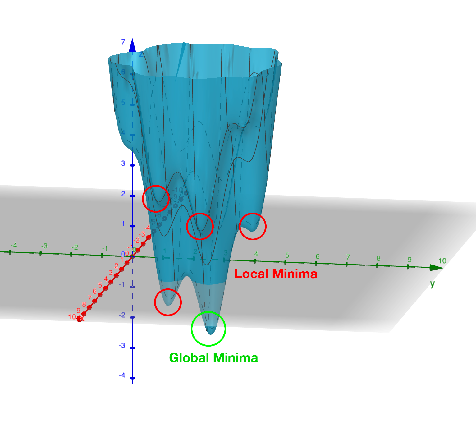
The problem, as it applies to evolving neural networks, is that some branch of the evolution - some set of structures which are formed by the process - may initially lower the fitness of the resulting network. It may take some time, several generations perhaps, for the topology to evolve sufficiently to discover that this new set of structures is able to explore a globally 'fitter' area of the solution space. Without some mechanism to protect this innovation, to give it time to see if it bears fruit, it will get removed from the population because of its inferior fitness.
So, NEAT needs to preserve novel developments for some period of time to allow the algorithm to explore far enough down these alleys to see if there’s value in them. You can think of it as a form of backtracking in the algorithm. NEAT achieves this with another concept from the natural world: Speciation.
In the animal kingdom species form a boundary to mating between organisms (a semi-permeable boundary, you could argue, by shouting MULES!) because of the mismatch between chromosome sizes or some other asymmetry. It’s the same in NEAT. We define some measure of compatibility between the genomes that encode our network topologies and only allow those members of the population who are compatible with each other are allowed to mate. In this way, as novel network structures appear through mating and/or mutation, NEAT can preserve these differences, allowing different branches of development to explore different areas of the solution space.
Organisms compete only with individuals within their species, not with the entire population. This is how NEAT protects innovation until it has a chance to prove itself.
Compatibility
Categorising organisms into groups which share similar topologies is another problem for which innovation numbers provide an elegant solution.
When we compare the genomes of two organisms the more disjoint and excess genes there are the less evolutionary history they share, meaning they’re less compatible. In practice, it’s not just disjoint and excess genes which are counted but also a measure of the average weight differences between matching genes.
The NEAT paper encodes the formula for compatibility in this magical spell:

Where E is the number of excess genes, D is the number of disjoint Genes, W is the average weight difference of the matching genes, c1, c2 and c3 are coefficients that allow to adjust the relative importance of the three factors and N is the number of genes in the larger genome (allowing us to normalise for genome size).
δ, then, is a measure of distance between two genomes. This means we can specify a threshold and compare each genome to each species one at a time. The genome is placed in the first species where the distance δ is less than the threshold, if it’s not placed in any species then a new species is created for it.
Again, the historical marking of topological structures with innovation numbers provides an elegant solution to what seemed like a tricky problem.
Why Use NEAT?
We’ve covered how NEAT works, and it’s cool and everything, but why would you use it rather than just copy/pasting some PyTorch code from ChatGPT? What’s the trade-off for the extra complexity involved? Is it better than anything else for solving any particular class of problem?
This is the conclusion from the original NEAT paper:
…evolving structure and connection weights in the style of NEAT leads to significant performance gains in reinforcement learning. NEAT exploits properties of both structure and history that have not been utilized before. Historical markings, protection of innovation through speciation, and incremental growth from minimal structure result in a system that is capable of evolving solutions of minimal complexity. NEAT is a unique TWEANN method in that its genomes can grow in complexity as necessary, yet no expensive topological analysis is necessary either to crossover or speciate the population. It forms a promising foundation on which to build reinforcement learning systems for complex real world tasks.
Stanley & Miikkulainen 2002
The stated aim of the paper was to prove that, when 'done right' (sic) an approach which evolved both the structure and the connection weights of a network would prove to be more performant than one with a fixed topology. The results in paper show that this is exactly what the authors found.
So, rather than a solution to some subset of problems where you’d use, say Reinforcement Learning, the paper contends that using NEAT will, most of the time, result in a more performant network. Furthermore, NEAT may well provide you with a more sophisticated solution than a static-topology approach can provide…
Again, from the original NEAT paper:
Strategies evolved with NEAT not only reached a higher level of sophistication than those evolved with fixed topologies, but also continued to improve for significantly more generations.
There’s also this interesting Stack Exchange question and answer that provides some advice on where NEAT can be useful. The author of one of the answers suggests that the form of NEAT’s fitness functions can provide some interesting options that can’t be achieved with gradient-based approaches. Interesting.
The trade-off for all this improved performance seems to be the size of the neural network required to provide a feasible solution. If it’s possible to approximate the target function with a relatively small neural network, NEAT could be worth a look.
That’s just with 'vanilla' NEAT, though. If it looks like standard NEAT isn’t a great fit then there are extensions to algorithm that may help.
Extensions and Improvements
Real-Time NEAT
What if there were a computer game in which you trained a set of soldiers - telling them how to behave (take cover when being fired upon, try to outflank the enemy with your own movements or by drawing them in, etc) after which you could watch how your team fare against a team trained by someone else. What if this game worked by evolving neural networks which acted as the 'brain' of each soldier. Each time a soldier did something you wanted them to do you rewarded them, each time they did something else you punished them and the network learned from this.
Well, in 2005 Stanley et al. did exactly this. And, helpfully, they published a paper which outlined how they did it - how they took the principles of the NEAT algorithm and applied them in a real-time setting.
Combined with the fact that NEAT seems to perform well at evolving gaits for robots, this presents some interesting avenues for further exploration. Imagine, for instance, that a robot exploring a remote area (deep ocean, perhaps, or an exo-planet) which becomes damaged in some way (a robot with jointed legs loses one of its legs or a leg becomes otherwise disabled), NEAT allows it to evolve the most efficient gait possible with the remaining limbs. Yes, you could evolve networks for multiple scenarios beforehand, but it might not be feasible to explore all possible scenarios. Also, this way you can take into account any unexpected environmental factors that weren’t known beforehand.
Hyper-Cube Encoding NEAT (HyperNEAT)
In their 2009 paper, breezily titled A Hypercube-Based Indirect Encoding for Evolving Large-Scale Neural Networks, Stanley, D’Ambrosio and Gauci introduced algorithm based on NEAT which addresses some of the issues with vanilla NEAT and provides help in creating networks which solve problems that have a spatial/geometric component.
I’ve previously talked about NEAT as mimicking biological evolution. This is true in the general sense but strictly speaking it’s not quite accurate. Think about it this way - the human body has more structures than the genome that encodes it. There’s no direct encoding between the genotype and the phenotype.
Furthermore, there are a lot of 'motifs' in the human body: left/right symmetry, fingers and toes, and the patterns of neural connectivity in the brain displays a form of repetition-with-variation, for example.
Lastly, a general issue with neural networks is they tend to discard spatial/geometric information about the structure of a problem - information that can be useful to the creation of an efficient solution. For instance, the squares on a chessboard (important, I think you’d agree), or the location of sensors on a robot - these are things that we, as humans, take for granted but which networks need to learn… unless that spatial information is encoded in the structure of the network itself.
Compositional Pattern Producing Networks
HyperNEAT addresses these issues by using an indirect encoding. Rather than encoding the neural network being evolved with a one-to-one mapping between genes in the genome and connections in the resulting network, HyperNEAT encodes the information about connections between nodes and the weights of those connections in another type of network called a Compositional Pattern Producing Network (CPPN). The CPPN is then queried for this information and the network is created.
CPPNs are a blog post topic all by themselves, but to give you an idea of how this works…
In HyperNEAT we refer to the network we’re evolving, the output of the algorithm, as the substrate. In vanilla NEAT the entire network topology is evolved by the algorithm. In HyperNEAT we need to define the potential structure of the substrate - how many layers of hidden nodes there are, for instance, and how many nodes in each of those layers - and HyperNEAT will tell us which of those nodes need to be connected to each other and the weights associated with the connections.
Defining the initial, potential structure of the substrate manually allows us to encode the spatial component of the problem in the geometry of the substrate. For instance, we might position the input nodes that represent sensors on a robot as a ring of nodes and the hidden layers as concentric rings inside the ring of input nodes.
Another example is the visual discrimination tasks that is described in the HyperNEAT paper itself. In this example each pixel which represents the image being displayed and interpreted by the network is represented as an input node in the substrate and all these input nodes are in positions which match the pixels they represent.
Painting Hypercubes
Once we’ve defined the substrate, HyperNEAT evolves a CPPN. If you imagine the CPPN as a flat plane of bounded size, each point on the plane represents a node in the substrate. If we query the CPPN for two points (x1, y1), (x2, y2) the CPPN will return us the weight of the connection between the two nodes represented by the two points.
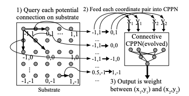
Think about it this way - image a flat, bounded plane and add perlin noise to it - a monochromatic cloud.
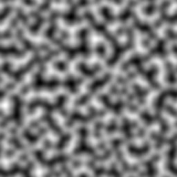
Then we have a field of pixels each of which has a colour value between 0 (black) and 1 (white). If we pick two points on the plane (representing two nodes in the substrate) and draw a line between them and sum all the values of the pixels on that line, we have the weight of connection between the two nodes/points.
Now, our CPPN has 4-dimensions (x1, y1, x2, y2) so rather than a plane we’re dealing with a 4-dimensional hypercube (hence the name Hyper NEAT). What HyperNEAT is doing is 'painting' the inside of this 4-dimensional hypercube, the thickness of the paint defines the connection weights between the nodes in the substrate.
Dynamic Dimensionality
Besides solving all the problems I listed above, HyperNEAT’s CPPN encoding provides another interesting side effect. If we have 100 nodes in our substrate, and we evolve a solution, and then we realise we need more nodes - for instance in the visual discrimination task we decide we need to increase the size and/or resolution of the input image - we can do so without further evolution! We can just query the encoding CPPN at the necessary points that represent the (normalised) locations of our new nodes on the substrate and Kablammo!, we get a more complex substrate from the same CPPN. Interesting.
For more detail on Compositional Pattern Producing Networks, especially their ability to encode different activation functions for network nodes (rather than just the usual sigmoid/guassian) take a look at Ken Stanley’s 2007 paper Compositional Pattern Producing Networks: A Novel Abstraction of Development
Evolvable Substrate HyperNEAT (ES-HyperNEAT)
ES-HyperNEAT was inevitable, really. I mean, we have an algorithm which can evolve neural network topologies, and we have an extension which evolves weights… how long was it going to be before someone got the chocolate mixed up with the peanut butter?
From the EPLEX ES-HyperNEAT page:
…the philosophy is that density should follow information: Where there is more information in the CPPN-encoded pattern, there should be higher density within the substrate to capture it. By following this approach, there is no need for the user to decide anything about hidden nodes placement or density. Furthermore, ES-HyperNEAT can represent clusters of neurons with arbitrarily high density, even varying in density by region.
I illustrated HyperNEAT with this idea of painting the inside of a hypercube. ES-HyperNEAT looks at the painting, finds those parts of the painting that have the most paint and adds structure there.
The way in which it finds the most-painted areas will be familiar to anyone who has worked on game-engines - specifically on optimising collision detection - Quadtrees.
Quadtrees
Take a 3-dimensional space (probably easier to imagine than >3) and split it into 4 equal parts, split each of those parts into 4 equal parts, then each of those into 4 and so on until you reach some predefined minimum volume for a part. Each of those parts at each level of granularity is tagged with the information density it contains.
This is the Division and Initialisation phase.
Next, the quadtree is traversed, depth first, until a quadtree node’s level of information is smaller than some threshold (or the quadtree node has no children) and a connection is created for each qualified quadtree node.
This is referred to as the Pruning and Extraction phase.
If you’re interested in diving deeper into the details of ES-HyperNEAT you can do no better than the original 2012 paper An Enhanced Hypercube-Based Encoding for Evolving the Placement, Density, and Connectivity of Neurons
Novelty Search
The approaches above add to the NEAT algorithm itself, Novelty Search is an approach which alters the implementation of the fitness function used during evolution to measure the performance of candidate networks.
Novelty Search is not specific to NEAT, it’s a metaheuristic in and of itself, but the application of Novelty Search in fitness functions has been explored and yielded some interesting results.
Around 2015 one of the authors of the original NEAT paper, Ken Stanley, delivered a series of talks to promote a book he’d written entitled 'Why Greatness Cannot Be Planned: The Myth of the Objective' in which he showcased some of the applications built with NEAT by him and his research students. For example, one of these applications, called 'PicBreeder' allowed visitors to a website to 'evolve' images. These images were created by networks evolved with NEAT and in the presentations Dr Stanley shows examples of images which resemble recognisable objects: faces, animals, furniture, vehicles, etc… He goes on to explain how these recognisable images are impossible to create deliberately. If you try to create something recognisable you will fail - you can only find them. They are a happy accident which lucky users of the system find from time-to-time.
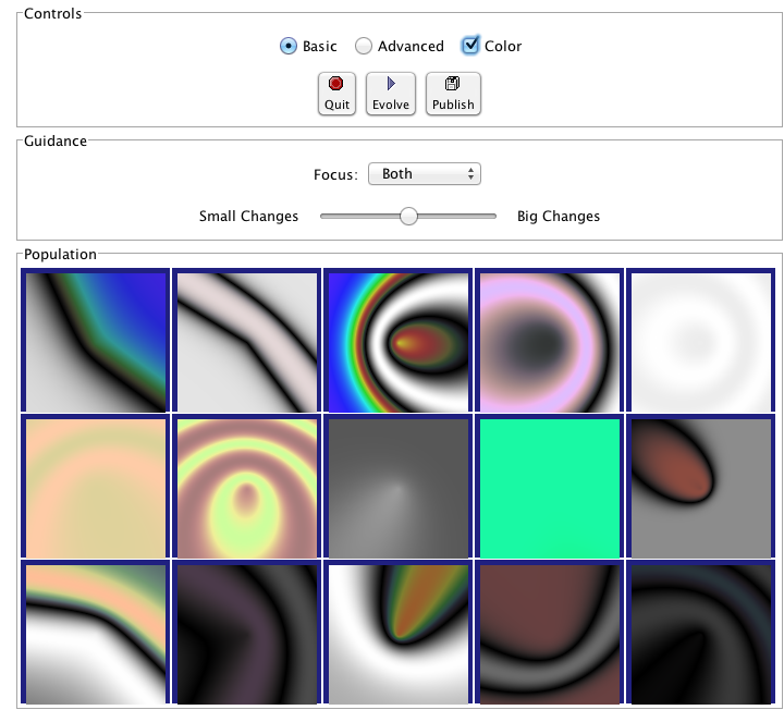
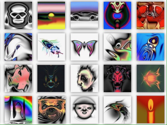
This idea of serendipity appealed to Dr. Stanley, it seems, and he took the idea of 'finding' these recognisable objects - so rare in the vast expanse of the possible search space reachable by the networks generating the images - and he dug deeper. What he realised was that if you tried to create a recognisable image - even if you had something you felt might be close to becoming a face, or an animal - you could never actually get there. However close you thought you were it would evolve in some other direction, there were just too many alternatives. The only way to come up with these rare events, these recognisable novelties, was to give up trying. The randomness of the system meant you were always doing something new, whether you tried or not you were unable to direct the process.
This is the fundamental idea behind novelty search - you direct the evolution to just do something novel, something it hasn’t done before, and then you see if that solves your problem.
Novelty Search is disarmingly simple - reward the network which does something new.
That’s it.
What he found by doing this was that networks which had their evolution guided by novelty search were able to solve problems which 'normal' fitness function weren’t able to solve. Novelty Search was also able to find solution to complex problems which were superior to those found through 'normal' fitness functions.
Here’s a video that gives a lot more detail and isn’t too long.
And here’s Ken Stanley delivering a longer presentation about the whole concept. It’s more conceptual, but well worth a watch. I’ve scrubbed forward through the preamble for you. (you’re welcome).
Some of the claims made may have been overstated. For instance, when tackling a maze like this:
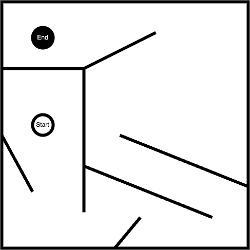
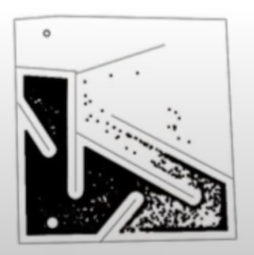
A naive fitness function would just look at the distance between the position of an agent and the 'end' marker and reward the network that produces the smallest distance. This results in a poor result as all the agents get caught in the local minima, unable to do what’s necessary and move away from the target in order to get around to the end.
An approach which rewards novelty does much better, it explores more of the map and finds the global optimum.
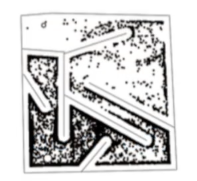
Dr. Stanley points out how novelty search is far more capable of finding a feasible solution. This may be true, but it requires a more compelling comparison, for sure. That being said, there are many compelling examples out there of novelty search outperforming the traditional fitness function. For instance, this example of the evolution of a biped gait.
It’s pretty clear which is the most successful approach, here.
Conclusion
Taking the time to find, read, and understand ideas explored in the past can be an entertaining enough experience. However, it can also yield fascinating topics for further exploration that, while niche, can be applied to problems we may be presented with here in the present.
The NEAT algorithm provides an elegant way of solving difficult problems and provides a means of providing compact, efficient neural network implementations capable of solving complex problems. The extensions to NEAT may yet yield further insights.
Keep mining the archives!
Resources
Implementations of NEAT
There are lots of implementations of NEAT out there. However, the nature of open-source software means that while there are many repositories to look at, there are few implementation which are working, complete and documented enough to use the for anything useful. Even the things that do work are works produced by academic researchers rather than professional software engineers so don’t expect things like thorough documentation, tests, performance optimisations, etc., etc.
The 'Implementations' section of the Wikipedia page for NEAT provides a good list. Rather than repeat them here I’ll just provide a little advice:
-
The original C++ version linked to the original paper doesn’t seem to be available anymore. There are a couple of GitHub projects that appear to contain that original code, though, I think the one that leaves the original code most-untouched is https://github.com/janhohenheim/stanley_neat
-
Take a deep breath before you look through the Java implementations, it’s 'academic code' which is a euphemistic way of saying… well… you’ll see for yourself.
-
SharpNEAT is AWESOME! There’s documentation (which is huge in and of itself), some YouTube videos from the author, there are a lot of examples and a lot of options and extensions to explore. If only it built on Mono (I’m assuming it doesn’t because it wasn’t around when Colin Green started the project way back in the mists of time,) so we could use it to create controllers for game entities in Unity :(
Other Useful Stuff
There are a lot of resources (and further links) available at the page of the Neural Networks Research Group at UC Texas to related projects, demos, etc.
The HyperNEAT page of the Evolutionary Complexity Research Group (EPLEX) at UCF has a ton of links to both the foundational research for HyperNEAT and papers that have explored the further development of the approach.
