Setting up a home energy monitoring system
Introduction
I had been using a Smappee system that came with the solar panel installation at home for about two years. It was installed back in July 2020 to monitor the electricity generation and consumption in our house when I noticed something odd. I used the neat Smappee iOS app to check the five-minute averages to monthly averages of the energy generated by the solar panels on our roof. The system was tracking 5 minute averages for a while until, all of a sudden, data older than two weeks was aggregated at a longer one hour interval.
Before August 8th I was able to track data with a granularity of 5 minutes, after that date the best I could get was one hour!
To illustrate the issue, let’s look at a couple of sample plots. The first one is an example of 5 minute average production and consumption data for one day (August 23, 2022):
The next one shows the same graphs over a period of 16 days (from August 8th till August 24th):
The graph shows the granularity changes from 5 minutes to 1 hour on August 8th.
The obvious question I asked myself was how to keep granular data longer, and I saw two options:
-
I could ask the company behind the system to reinstate the longer data retention period.
-
I could investigate if I could build an energy monitoring system that would allow me to configure the data retention policy as I wished it to be.
I chose the second option, as it seemed to give me an opportunity to learn technologies I had never used before.
Before I found out about the data granularity issue, I had already discovered that the Smappee energy management system was quite open. It provides two ways to get access to the collected data. One method is to use the Smappee REST API, the other is to use MQTT.
The REST API can query endpoints in the Smappee Cloud, linked to an individual Smappee monitoring system located, for example, in one’s house. Use of the API is free for non-commercial use and requires setting up OAuth2 authentication.
When using MQTT, the Smappee monitoring system configuration has to be tweaked to point to a so-called MQTT Broker. Once that’s done, the Smappee device will send measurement samples at a once per second interval to the MQTT Broker.
The first access method polls data from the Smappee Cloud, while the second pushes data to a server.
With all this in mind, let’s consider the project goals I set for my Home Energy Monitoring System (HEMS).
Project objectives
The primary aim of the HEMS project was to collect Smappee data at specific aggregation levels and retention periods. Also, we want dashboards that display selected aggregates over a chosen time period.
For example, a Smappee, when configured to send data to an MQTT Broker sends data at a one-second interval. One may want to aggregate this data at minutes, days, weeks, or months intervals. Each aggregation level may have specific data retention periods. For example, we may keep the high frequency 1-minute aggregates for a few months. On the other side of the spectrum, we may keep indefinitely the monthly averages (and obviously, as long as storage capacity permits).
As I wanted my solution to be independent of external factors (such as the Smappee Cloud) as to not be exposed to the whims of external parties, I chose the MQTT route for building my HEMS.
Next to the already cited main objective, there were other objectives I wanted to achieve:
-
If possible, implement the system without any programming.
-
Use Free Open Source Software (FOSS) only.
-
Capture all knowledge gained in building the system as to make it easily reproducible.
-
Simplify installation with automation.
We’ll evaluate project objectives in the upcoming sections, but before we do that, let me give you a quick overview of the upcoming sections in this blog post:
-
A brief introduction to Smappee: describes the hardware that is at the centre of the data acquisition.
-
HEMS Architecture & Implementation: the application architecture and the mapping to a concrete implementation.
-
System provisioning: describes how the setup is industrialised using cloud-init and jinja templates.
-
Configuring Telegraf: raw data measurements need to be transformed before being written to a database, a task that is performed by a component named Telegraf.
-
Before I summarise some ideas about Future work at the end of the article, we dive into the different The Grafana Dashboards that I built in this project and the insights these provide me.
A brief introduction to Smappee
Smappees come in different versions of which I currently have two at home:
The first one, a Smappee Solar came with the solar panel installation and measures the total electrical power consumption of the house and the output power of the solar panels on the roof of the house. The second one is a modular Smappee Infinity that consists of:
-
a Smappee Power box that powers all connected Smappee devices and that measures line voltage(s). It supports both mono-phase and tri-phase power systems.
-
a Smappee Genius which is the "brain" of the system. This device implements Wifi and physical Ethernet connectivity and acts as a Gateway.
-
one or up-to 7 Smappee CT Hubs that each can measure current in up-to 4 electrical circuits.
The Smappee Power box powers the Smappee Genius, which is connected to the daisy chained CT Hubs via RS-485, using 4-wire twisted pair cables. These cables serve two purposes. First, they transfer power to the different Smappee components. Second, they form the communication channel between the Smappee components.
As mentioned in the introduction, a Smappee performs measurements at a 1 Hz rate. The Smappee genius measures:
-
Mains frequency (Hz) and mains voltage(s) (V)
-
Circuit currents (A)
-
Real Power (W), Reactive Power (VAR), Apparent Power (VA), and Power factor
The Smappee Solar is a scaled down version of the Smappee Infinity system optimised for Solar panel installations.
Even though the physical installation is best performed by a professional, anyone with basic IT skills can do the configuration.
I’ve had the Smappees in service for 3 years (Smappee Solar) and 9 months (Smappee Infinity) and both have proven to be very reliable and accurate systems.
HEMS Architecture & Implementation
Architecture
As mentioned in the introduction, I opted for MQTT as a means to access the Smappee data measurements.
The Smappee documentation says the following about using MQTT:
"Use of MQTT requires programming knowledge."
Interesting, and unexpected, so worth investigating.
The HEMS system needs to have the following components:
-
A Time-Series database that will store aggregated measurements with an optional data retention time.
-
A Display server that will offer various dashboards. The latter can be displayed using a web browser.
-
An MQTT Broker. It acquires raw measurements from Smappee and offers them to subscribers.
-
The raw Smappee measurements are most likely not in a format that is suitable to write to the time-series database as-is. We may want to only keep data we’re interested in and drop other stuff. Also, it is likely that we want to rename certain data fields. Therefore, we need a component that:
-
Subscribes to topics on the MQTT Broker.
-
Transforms and aggregates the raw measurements.
-
Writes it to the Time-series database.
-
Let’s call the last component the IO/transformer/aggregator.
Mapping of the architecture to specific components
Various alternatives exist for each component mentioned earlier, but I selected these (FOSS) implementations:
-
Time Series Database: InfluxDB
-
Display server: Grafana Server
-
MQTT Broker: EMQX
-
IO/Transformer/aggregator: Telegraf
I used a Raspberry Pi with Ubuntu Server Operating System to run these components as I have great experience with this combination.
The following diagram shows the overall set-up of the HEMS:

Let’s walk through the elements in this diagram one by one.
The electricity system
The electricity system in the house is comprised of:
-
A connection to the electricity grid and depicted as a lightning bolt.
-
An analog electricity meter. Note that this meter measures actual power and it will turn backwards when the energy production is higher than the consumption.
Note: in Belgium, all domestic consumers will be required to have a digital electricity meter by January 1st, 2025. This means that Fluvius, the company in Belgium that is responsible for tracking energy consumption, will have access to real-time meter readings and electricity consumption and injection can be billed separately.
The Smappee systems
-
A Smappee Solar that measures total energy consumption and total solar energy production.
-
A Smappee Infinity that measures energy consumption of individual electrical devices or groups thereof. Examples of the former are the electric oven and dish washer. Wall sockets are grouped already and are an example of the latter.
The Home Energy Monitoring System
-
A Raspberry Pi 4 Model B/8GB with a 250GB SSD (SATA disk connected to one of the Pi’s USB-3 ports via a USB-SATA converter).
-
The software components — EMQX MQTT Broker, Telegraf, InfluxDB server, and Grafana Server with data flowing from left to right.
-
An MQTT client — mainly used during debugging the MQTT/Telegraf configuration. The EMQX project has an MQTT client with a Graphical User Interface named MQTTX, but due to it being pretty slow, I switched to Mosquitto CLI.
-
I added the Raspberry Pi OS Metrics Telegraf configuration and Grafana Dashboard to monitor the Raspberry Pi.
With this out of the way, let’s look at configuration and system provisioning in the next sections.
System provisioning
It is a well-established fact that the Internet provides a wealth of information about setting up IT infrastructure and software. Obtaining accurate and up-to-date information can be a challenge though.
For example, take the absolutely great Raspberry Pi Grafana dashboard developed by Jorge de la Cruz. I installed and configured this component before tackling the energy monitoring part. When I added the latter, the Raspberry Pi monitoring dashboard stopped working. An analysis showed that the Telegraf configuration for the Raspberry Pi system monitoring was too generic and had to be tweaked.
Another challenge I faced was determining what software component versions are supported by a particular operating system. As I am using Ubuntu Server OS, two versions, 20.04 and 22.04 were suitable candidates, with a preference for version 22.04. Unfortunately, at the time I installed the system, EMQX was only supported on 20.04, which made 22.04 a no-go (at the time of writing EMQX on Ubuntu 22.04 is supported and I’m already running it on a test system).
A way to avoid having to go through a debugging cycle when provisioning a system is to use tools to automate the process as much as possible. Various alternatives exist, but I went for cloud-init.
As Ubuntu Server bundles cloud-init, we can use it to our advantage. We can provision a new system in a reproducible way, and we can do so in the fastest way possible. Compared to a manual installation and configuration, at least an order of magnitude faster. We can provision the HEMS system in the time span of about 12 minutes. SD card flash time is consuming a sizeable fraction of the total time.
In fact, after having gone through several iterations, I found out that we can optimise it further. Even though Ubuntu 20.04 doesn’t support booting of an external SSD, it still does so provided that there’s a bootable SD card installed on the Pi. The net effect is that the SD card needs to be flashed just once and only the SSD needs to be re-flashed. Given that it takes about 18 seconds to do this, we shortened the provisioning process down to 7 minutes!
Ubuntu 22.04 supports direct booting of an external SSD obviating the need to have an SD card installed on the Pi.
I plan to upgrade my current production system to the latest and greatest somewhere down the line. Have a look at Future work for a list of ideas.
Configuring MQTT on the Smappees
We can configure a Smappee to send its measurements to an MQTT Broker in the advanced configuration menu of the Smappee. For this configuration, we need the IP address of the broker and the port number it is listening on (default = 1883).
The following screenshot shows the advanced configuration screen of a Smappee.
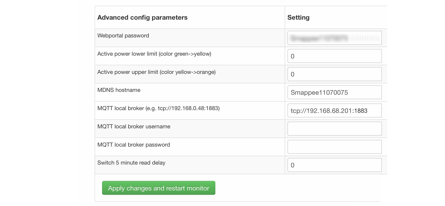
Note that the configuration set the broker’s IP address to 192.168.68.201, the port number to 1883, and the transport layer communication protocol to TCP.
With that configuration change, each Smappee will now start sending MQTT data to the broker. Note that we will lose data if the configuration is incorrect (e.g. wrong IP address or port number). Also, if the broker is down or unreachable, data will be lost.
MQTT sends data on so-called MQTT topics. Different options exist for encoding the actual data, but Smappee opts for JSON encoding.
The structure of the data is different between the Smappee Solar and the Smappee Genius. Let’s start with the Solar and then look at the other.
$ mosquitto_sub -h 192.168.68.201 -p 1883 -t servicelocation/f960f45d-c43b-4937-a8d0-ce1869206011/realtime| jq
{
  "totalPower": 255,
  "totalReactivePower": 251,
  "totalExportEnergy": 0,
  "totalImportEnergy": 807413694,
  "monitorStatus": 0,
  "utcTimeStamp": 1683799083538,
  "channelPowers": [
    {
      "ctInput": 1,
      "power": 1175,
      "exportEnergy": 6848910,
      "importEnergy": 884498523,
      "phaseId": 1,
      "current": 49
    },
    {
      "ctInput": 2,
      "power": 255,
      "exportEnergy": 0,
      "importEnergy": 807413694,
      "phaseId": 2,
      "current": 15
    }
  ],
  "voltages": [
    {
      "voltage": 241,
      "phaseId": 0
    }
  ]
}
On this device, the data we’re interested in are the line voltage (voltages/voltage), the two power readings (channelPowers/power for channelPowers.ctInput = 1 and channelPowers.ctInput = 2), and the timestamp of the measurement. We will explain later how this data is extracted and transformed before writing it to InfluxDB.
For the Smappee Genius, the (abbreviated) data looks as follows:
$ mosquitto_sub -h 192.168.68.201 -p 1883 -t servicelocation/5aaf6e89-89cb-4e33-bf34-05abc62f5563/realtime| jq
{
  "totalPower": 0,
  "totalReactivePower": 0,
  "totalExportEnergy": 5900400,
  "totalImportEnergy": 3332883600,
  "monitorStatus": 0,
  "utcTimeStamp": 1683799714000,
  "measuredFrequency": 49983008,
  "channelPowers": [
    {
      "publishIndex": 0,
      "formula": "$5500053415/0$",
      "power": 84,
      "exportEnergy": 2188800,
      "importEnergy": 280227600,
      "phaseId": 0,
      "current": 4,
      "apparentPower": 90,
      "cosPhi": 93
    },
    {
      "publishIndex": 1,
      "formula": "$5500053415/1$",
      "power": 7,
      "exportEnergy": 900000,
      "importEnergy": 277783200,
      "phaseId": 0,
      "current": 1,
      "apparentPower": 21,
      "cosPhi": 33
    },
    <elided>
  ],
  "voltages": [
    {
      "voltage": 242,
      "phaseId": 0
    },
    <elided>
  ]
}
The Smappee Genius collects more information than its smaller sibling. Observe the measuredFrequency measurement (expressed in µHz) which allows us to track the mains AC frequency, channelPowers.cosPhi, measures the so-called Electrical Power Factor (also known as cos(φ)) or power factor on a per channel basis. Interesting to note is the presence of the CT Hub Id and channel number in the channelPowers.formula value. This Id is a 10-digit number that uniquely identifies each CT Hub.
The following diagram shows the physical configuration & measurement points on the Smappee Infinity system.
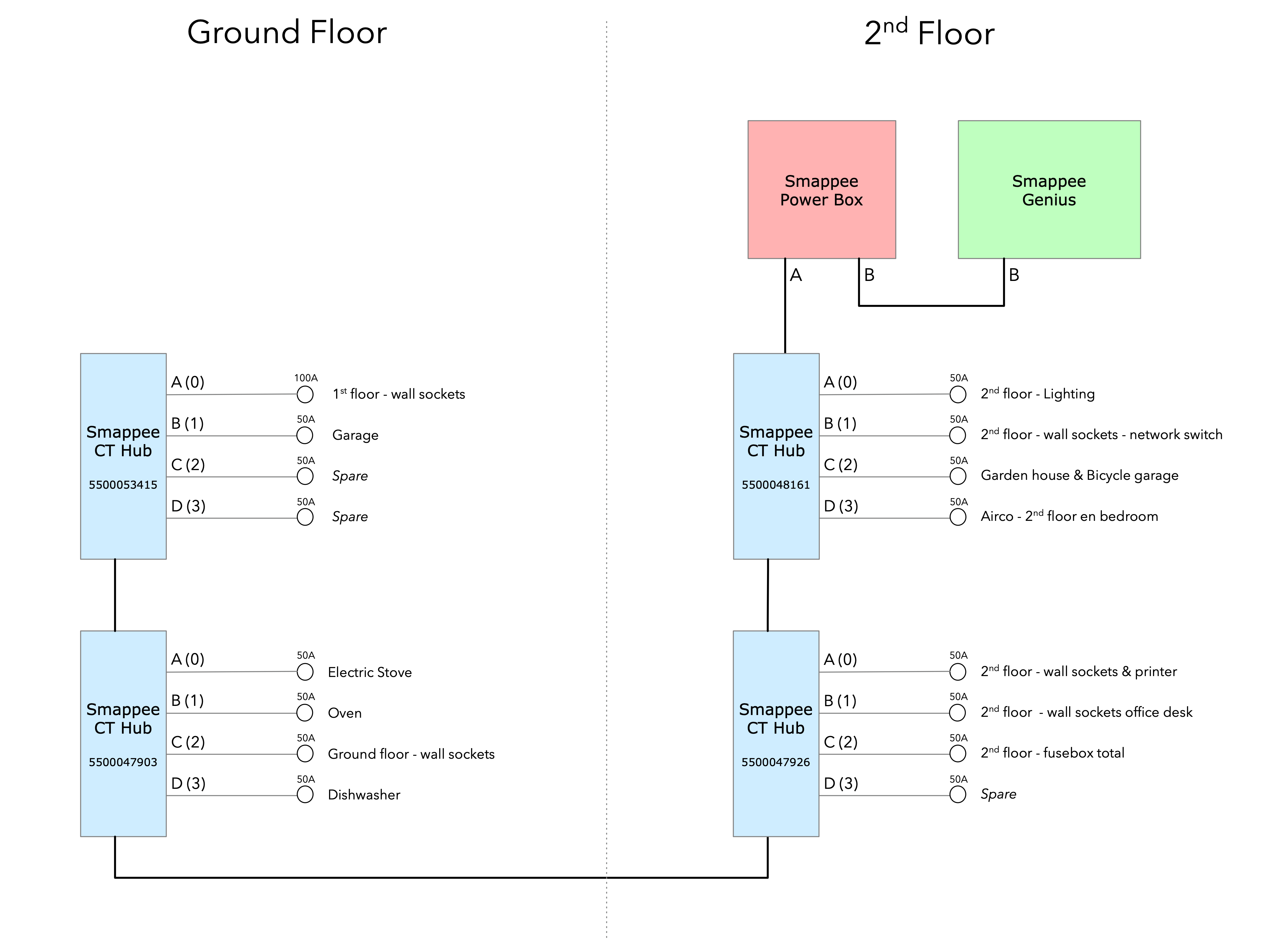
We recognise the four CT Hubs with their respective Id and what each CT Hub channel measures. The labels Ground Floor and 2nd Floor at the top of the diagram refer to the location of the fuse panel in which the Smappee components are located.
Now that we know the message format of the raw data published via MQTT, we will look at how we can get the messages into the Time series database.
Configuring Telegraf
Telegraf offers a series of plugins that fall into four categories: Input, Processor, Aggregator, and Output. Telegraf plugins that are relevant to our use case are:
-
Input: MQTT Consumer and the JSON v2 parser. The JSON v2 parser is a generic component that can apply to any input plugin.
-
Aggregator: Basic Stats
-
Processor: Regex
-
Output: InfluxDB v1.x
Reading and transforming the MQTT data sources
Our two Smappees send data to the EMQX MQTT broker located at tcp://192.168.68.201:1883. Let’s look at the relevant part of the Telegraf configuration for the Smappee Genius.
[[inputs.mqtt_consumer]]
  alias = "smappee-2"
  name_override = "smappee-data-2"
  servers = ["tcp://192.168.68.201:1883"]
  topics = [
    "servicelocation/5aaf6e89-89cb-4e33-bf34-05abc62f5563/realtime"
  ]
  # The "host" tag is irrelevant in this use case. Drop it
  tagexclude = ["host"]
  data_format = "json_v2"
  [[inputs.mqtt_consumer.json_v2]]
    [[inputs.mqtt_consumer.json_v2.field]]
      path = "channelPowers.#(formula==$5500048161/0$).power"
      rename = "2nd-floor-lighting"
      type = "float"
    [[inputs.mqtt_consumer.json_v2.field]]
      path = "channelPowers.#(formula==$5500048161/1$).power"
      rename = "2nd-floor-wall-sockets-network-switch"
      type = "float"
    [[inputs.mqtt_consumer.json_v2.field]]
      path = "channelPowers.#(formula==$5500048161/2$).power"
      rename = "garden-house-bicycle-garage"
      type = "float"

  <elided>
We are configuring the mqtt_consumer input plugin and point it to connect to the EMQX broker. The topics settings is used to instruct the plugin to subscribe to the MQTT topic of interest. Next, the name_override setting is used to name the stream of data elements produced by the input plugin. This name is used to select the desired route that the data will follow as other plugins process it. Finally, the data is in JSON format (json_v2) and we exclude the host field.
We’re ready to configure the JSON parser, which is done in the inputs.mqtt_consumer.json_v2 configuration section. For each field in the data that we want to retain for further processing, there’s a section that selects the field, renames it, and specifies its format.
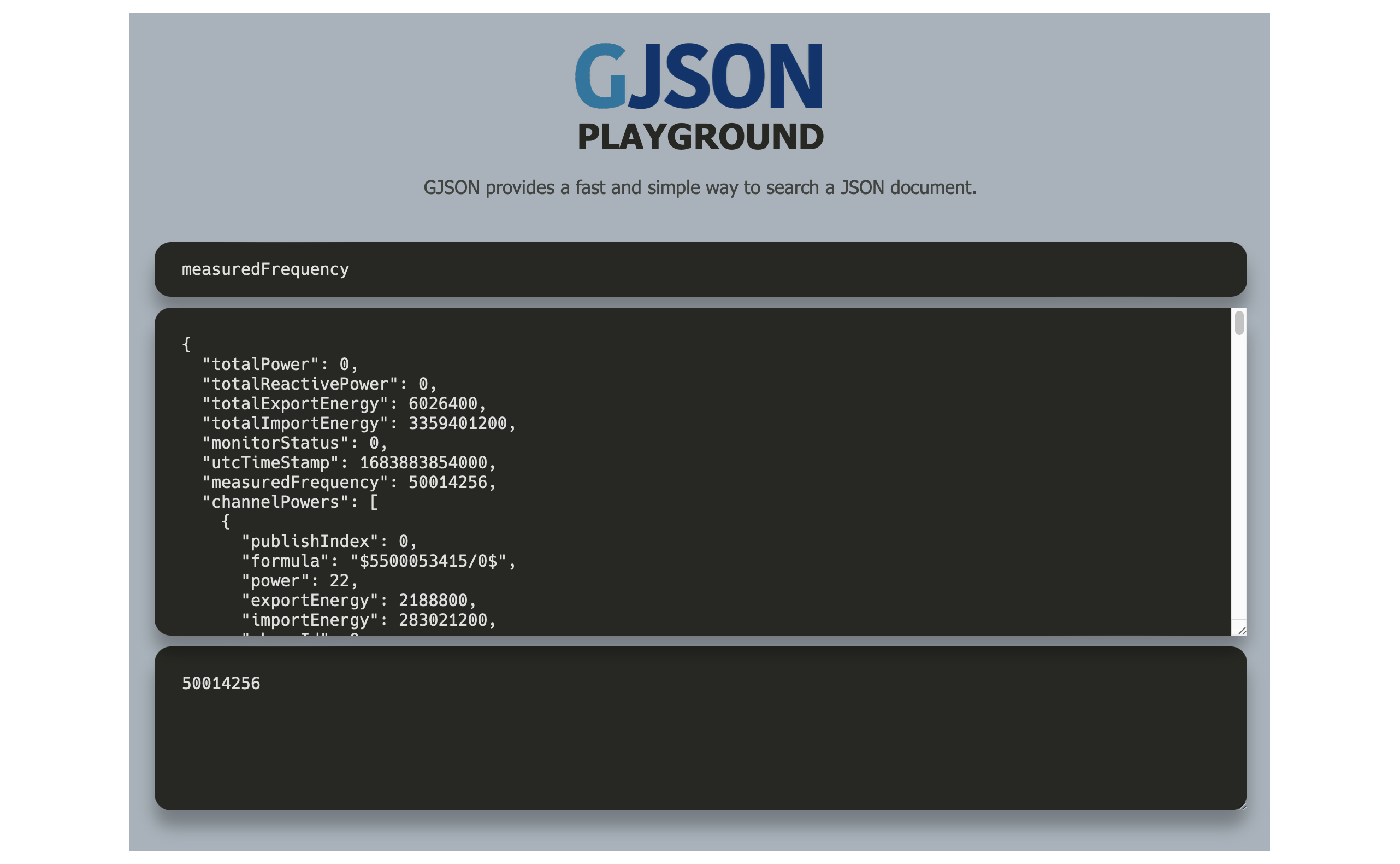
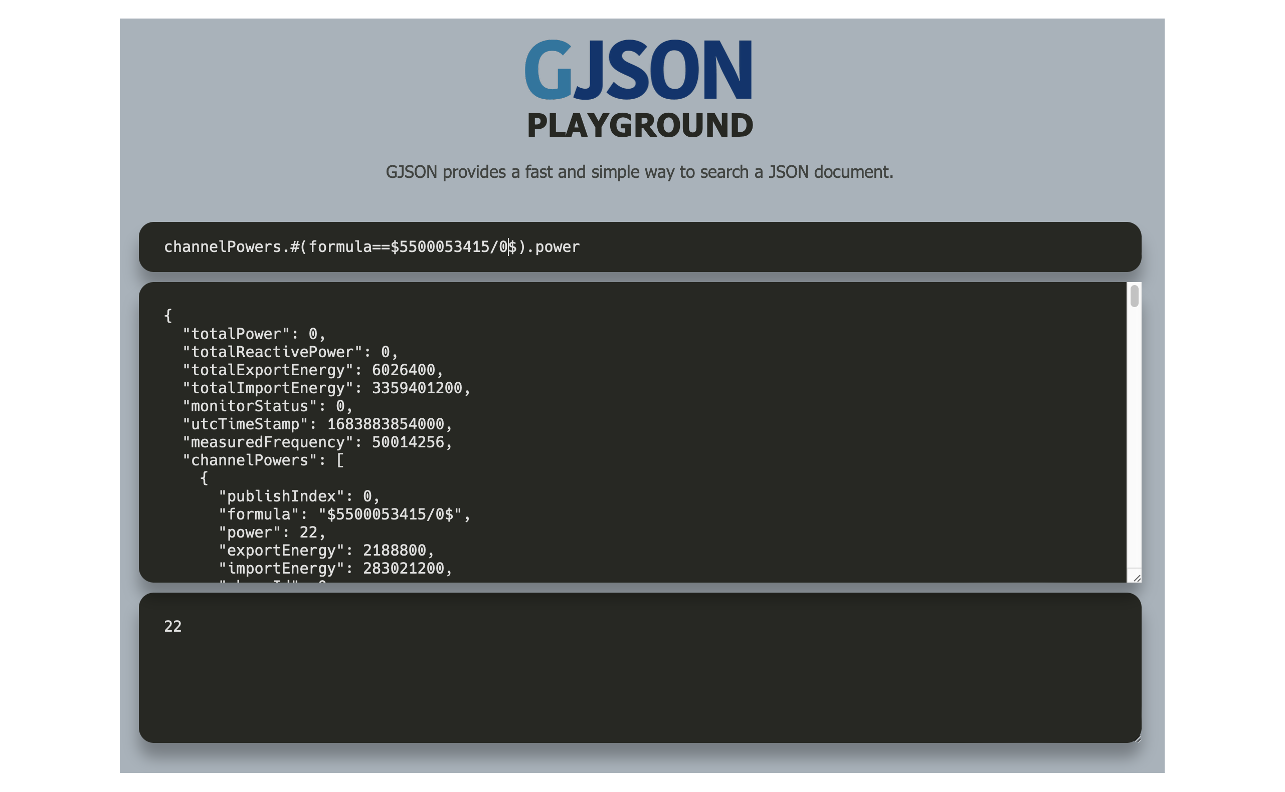
You may wonder how one knows the syntax of the path selector. A very handy tool for this is the GJSON playground which allows one to try out queries on JSON data. It comes with examples for the most important use cases.
Here are two examples of queries on the Smappee Genius data. These respectively extract the measuredFrequency value and the power value for channel 0 on the CT Hub with Id 5500053415.
Transforming the MQTT topic
If we would limit the Telegraf configuration to what we have up to now, the data would be tagged with the rather lengthy topic (servicelocation/5aaf6e89-89cb-4e33-bf34-05abc62f5563/realtime). It makes sense to drop the servicelocation and the realtime parts. We can do this using the regex processor by adding the following configuration.
[[processors.regex]]
  namepass = ["smappee-data-2"]
  [[processors.regex.tags]]
    key = "topic"
    pattern = ".*/(.*)/.*"
    replacement = "smappee/${1}"
We can observe:
-
By specifying the
namepasssetting, the processor will only apply to the data we want to transform. If we would leave it out, the transformation would be applied on all data. -
We select the
topickey and apply a pattern match on its value via a regular expression which captures the value of the second field. -
The original topic value,
servicelocation/5aaf6e89-89cb-4e33-bf34-05abc62f5563/realtime, is replaced by the new valuesmappee/5aaf6e89-89cb-4e33-bf34-05abc62f5563.
Aggregating the data
Writing the measurements at the Smappee 1Hz sample rate is overkill, so we want to aggregate measurements at a longer interval. I kept average values over 1-minute intervals. We can implement this using the basicstats Telegraf aggregator plugin.
Here’s the configuration for this:
[[aggregators.basicstats]]
  namepass = ["smappee-data-2"]
  ## The period on which to flush & clear the aggregator.
  period = "60s"

  ## If true, the original metric will be dropped by the
  ## aggregator and will not get sent to the output plugins.
  drop_original = true

  ## Configures which basic stats to push as fields
  stats = ["mean"]
The usage of the namepass setting should be familiar by now. Other than that, we set the aggregation interval to 60 seconds (setting period) and we drop the original (1 second) measurements as we only want the plugin to calculate the average value via the stats setting.
We could also choose to let Telegraf handle further aggregation to longer intervals, but that’s a task that is better left to InfluxDB as the latter will also help use to specify data retention times.
All that’s left to do is to write the data to the Time series database.
Writing the processed data to InfluxDB
An InfluxDB server is running on the same host (http://192.168.68.201:8086). The only thing missing is the Telegraf InfluxDB output plugin configuration:
[[outputs.influxdb]]
  namepass = ["smappee-data-2"]
  alias = "smappee-out-2"
  urls = ["http://192.168.68.201:8086"]
  database = "smappee_monitoring_2"
  username = "this is not my username"
  password = "this is not my password"
This configuration is for InfluxDB version 1. We should not pass the database username & password in the config. I will revisit this as part of a future migration to InfluxDB version 2, which has a completely revised security implementation.
Lessons learned from setting up Telegraf and InfluxDB
Telegraf - message routing through plugins
The Telegraf plugin system is powerful, but it took me quite some time to wrap my head around its configuration. Even though there are video tutorials and online courses on various Telegraf related topics, it took me a lot of time to grasp how data is routed through the system by applying the name_override, namepass, and namedrop parameters. When it finally dawned on me how it works, it looked trivial (and it actually is).
Telegraf - plugin application order
The order of application of Telegraf plugins is:
-
Input plugins
-
Processor plugins
-
Aggregator plugins
-
Output plugins
For Processor plugins, we can tweak the order of execution by setting the order parameter on all processors involved.
The Telegraf configuration document is worth reading and provides a lot of very useful information that you may want to read before embarking for the first time on a Telegraf project.
Telegraf - conclusion
The HEMS has a relatively simple Telegraf configuration. The configuration can be put in a single file (/etc/telegraf/telegraf.conf), or across multiple files located in the /etc/telegraf/telegraf.d folder. An advantage of using multiple configuration files is that the configs for different Smappee systems can be logically separated. In fact, when I recently added some Zigbee 3.0 devices that connect to a Zigbee2MQTT bridge configured in a Home Automation system, its Telegraf configuration was stored in a dedicated file. One thing to be aware of is that using multiple configuration files doesn’t introduce any separation between the individual configs, so treat it as if everything was stored in a single file.
A cool feature of Telegraf is that a template configuration file can be generated by the Telegraf CLI for a given list of Telegraf plugins. This configuration includes all possible settings applicable to the chosen plugins.
I think that in a complex system, it’s challenging to maintain the Telegraf configuration(s). InfluxDB version 2 probably has features that simplify managing this, but that’s something I haven’t explored yet.
InfluxDB
Installation and configuration of InfluxDB version 1 is simple. I automated the installation using cloud-init, including the creation of the user databases & user account.
I spent little time securing the set-up as I think InfluxDB version 2 has a lot more to offer.
Actually, when I started this project, I wasn’t aware of the fact that there is a version 2 of InfluxDB. I found out by the time the project was already long underway. I did a small trial by uninstalling version 1 followed by an installation of version 2. What I found impressive is that when I started the version 2 instance for the first time, it told me it had detected version 1 databases and if I wanted them converted to version 2. I accepted the offer and it worked flawlessly. What I liked even more is that when I reverted the installation to version 1, my original data was still there and ready to continue where I left off. A really refreshing experience!
Provisioning the HEMS system with cloud-init
cloud-init is a method for cross-platform instance initialisation. We can utilise it even on bare-metal installations like on a Raspberry Pi. It performs user creation, can execute custom scripts, installs packages, creates files, partitions disk, creates file systems, etc.
It used to have rather poor documentation, but this is a thing of the past. When you want to start with cloud-init, have a look at the Cloud Config Examples which should get you started quickly. These examples are part of the Reference Documentation on the cloud-init website.
Using cloud-init
I started using cloud-init many years ago on another Raspberry Pi project. Back then, I used the Hypriot operating system (a derivative of Raspbian) which has integrated support for cloud-init and Docker. The Hypriot FOSS project has gone dormant since a few years, but one of the core contributors pointed out that Ubuntu Server has the same goodies incorporated. I switched to Ubuntu and never looked back.
A cloud-init deployment is driven by a cloud-config file in YAML format. You can find the configuration for this project here. It’s part of the HEMS GitHub repository that also contains the Telegraf configuration smappee-2.conf for the Smappee Genius and smappee.conf for the Smappee Solar.
Noteworthy mentioning is that cloud-init supports instance data with jinja template rendering. Instead of directly applying configuration settings in the cloud-config file, metadata comprising key/value pairs can be passed to cloud-init in a file and these can be de-referenced in the cloud-config file.
For the Ubuntu cloud-init installation, I adapted the Hypriot flash command supports passing in the metadata file during flashing. You can find this version here.
Here’s an example invocation of the command to flash an SSD (or SD) with Ubuntu 22.04
$ flash -n home-iot -j -m cloud-init/meta-data -u cloud-init/smappee-2.yml \
  https://cdimage.ubuntu.com/releases/22.04/release/ubuntu-22.04.2-preinstalled-server-arm64+raspi.img.xz
Conclusion
The Project objectives set at the start of the project were all achieved.
No programming was required to build the HEMS. All software components are FOSS, and we can provision a new HEMS system in a matter of minutes in a reproducible way.
Apart from provisioning the HEMS, the only thing that needed to be changed was to configure the Smappees to send their data to the MQTT Broker.
Finally, and that’s about the only manual step, we configure Grafana data sources and import Grafana dashboards.
The Grafana Dashboards
Up to now, this article has focussed on the HEMS implementation. Let’s shift to the Grafana dashboards I created and the insights these give into the energy production and consumption in the house.
The Energy production and total Energy consumption dashboard
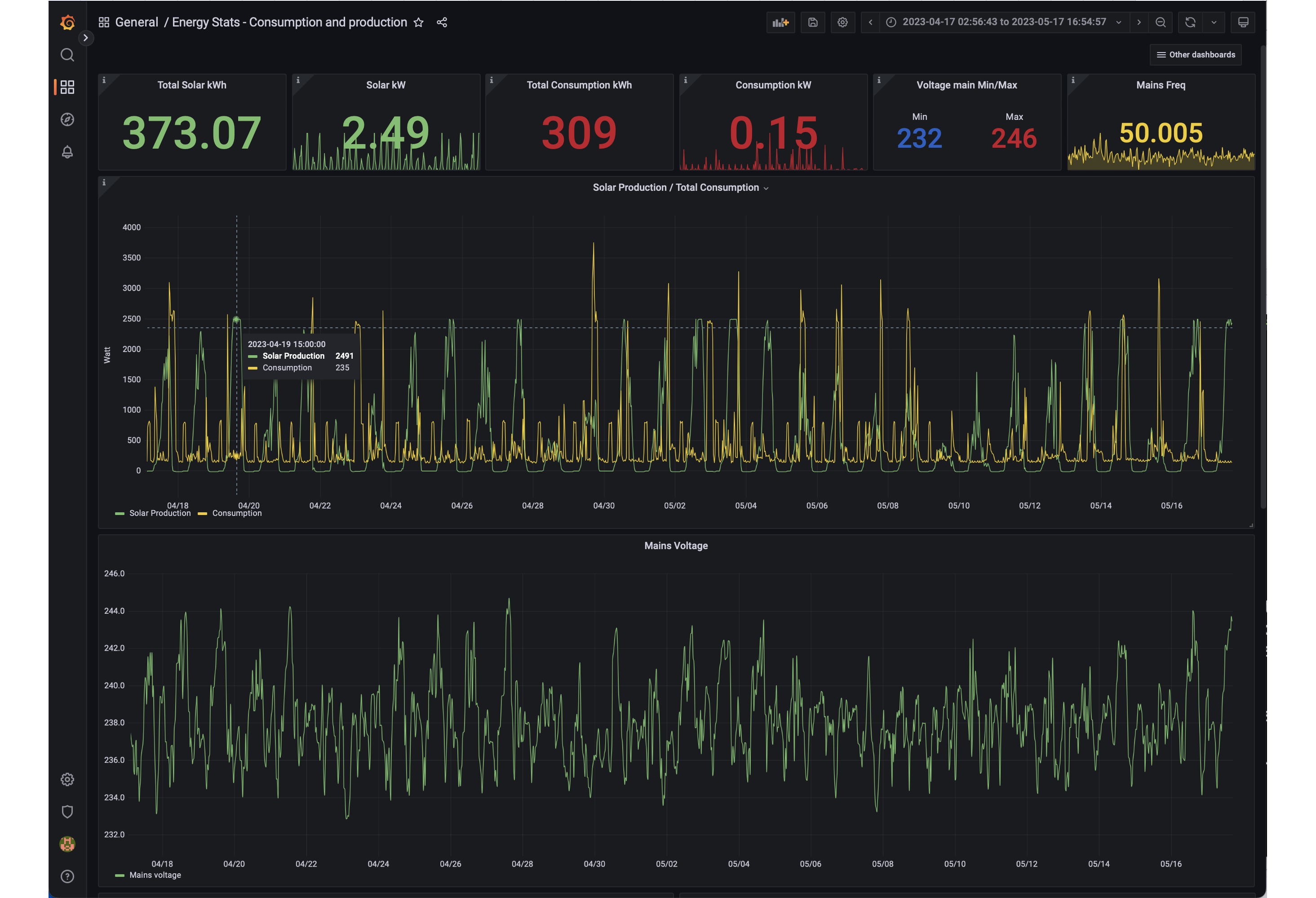
The Smappee Solar measures energy production, total consumption, and the mains voltage. This brings us to the first Grafana dashboard that displays this information in a couple of panels, as shown here:
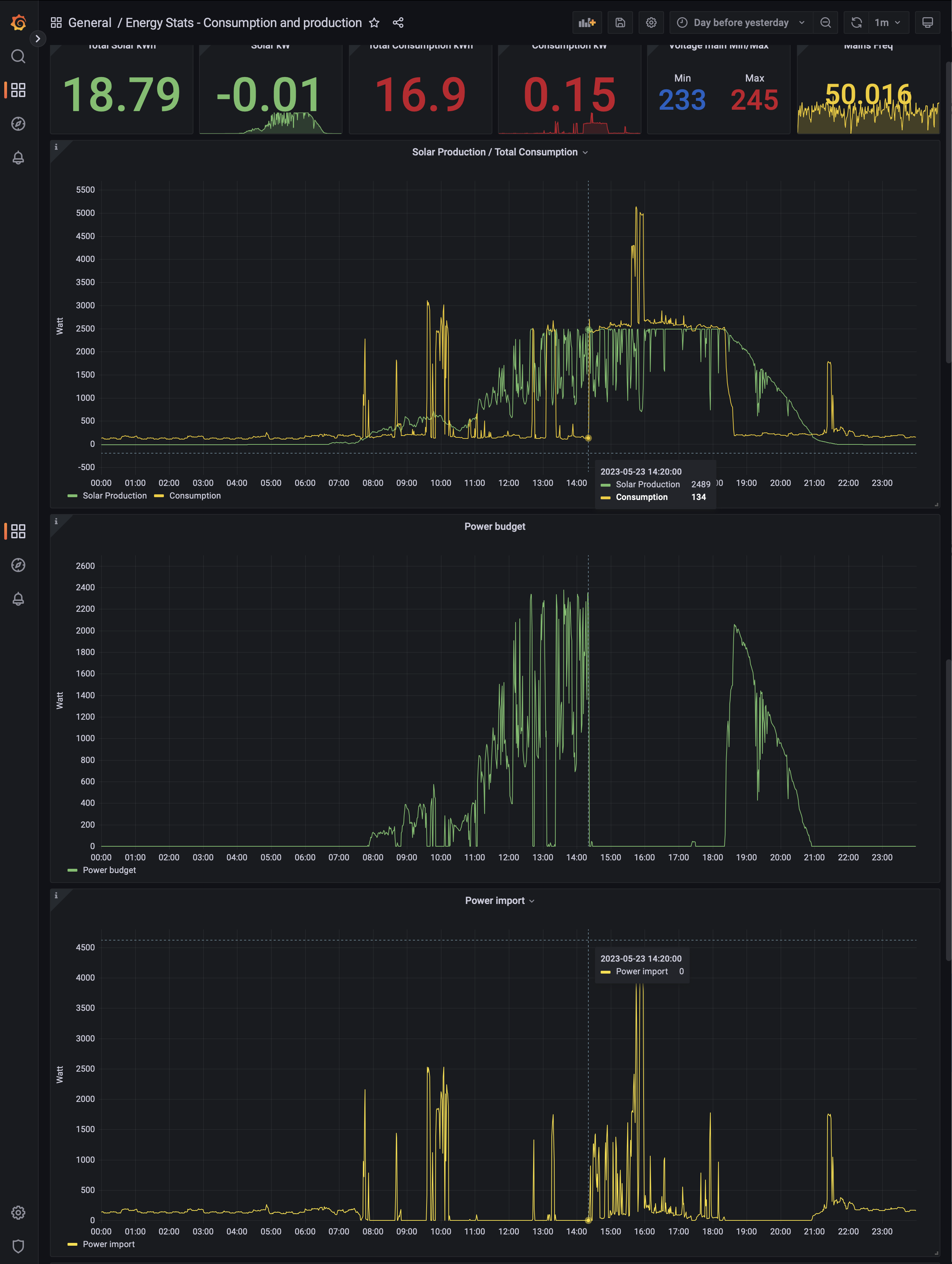
The six status panels at the top display the following information:
-
Total solar energy generated over the selected time period in kWh.
-
Average solar power generated in kW over the last minute.
-
Total energy consumption over the selected time period in kWh.
-
Average total energy consumption in kW over the last minute.
-
Mains voltage minimum and maximum value over the select time period in Volts.
-
Mains frequency in hertz (this value is measured by the Smappee Genius).
Next up are three line graphs showing one-minute average values for:
-
Electricity production and total consumption
-
Power budget
-
Power import
The last two graphs display values that are not directly measured, but are derived in Grafana from the data displayed in the first graph.
Even though the installed Solar panel capacity is about 4 kW, the production capacity is capped to 2500 W by the lower rated power of the inverter attached to the panels.
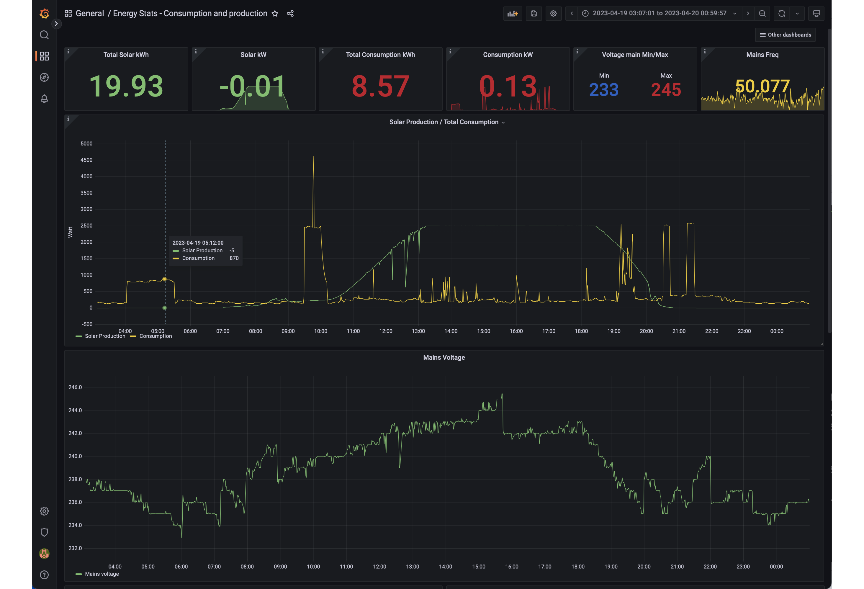
The Grafana dashboard allows us to quickly answer questions like:
-
What is the total amount of energy produced by the solars panels?
-
What is the peak power produced by the solar panels?
-
What is the total amount of energy produced by the solar panels during ramp-up in the morning till 13:00?
-
What is the total amount of energy produced by the solar panels for the remainder of the day?
The top-left status panel tells us that the answer to the first question is 18.79 kWh. The second question is answered by hovering over the first graph during a moment at which maximum output is generated:
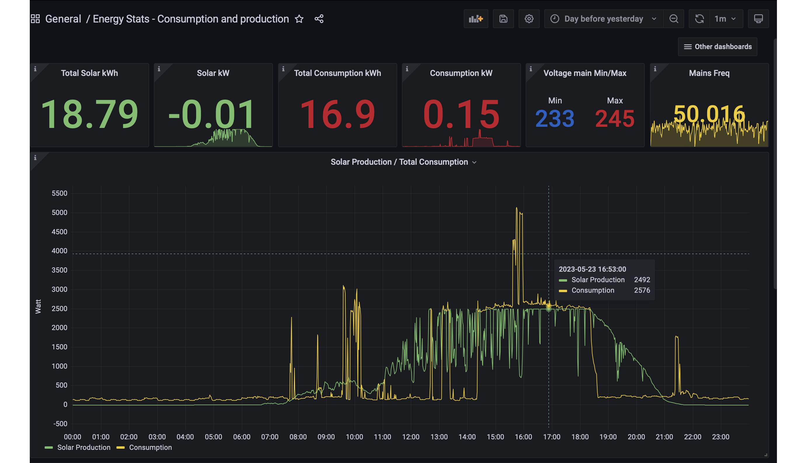
The answer is 2492 W, which corresponds to the rated power capacity of the installed inverter.
We can answer the other two questions by zooming in on the selected time spans in the dashboard. We can then read the values in the first panel on top of the dashboard. Let’s see what this gives.
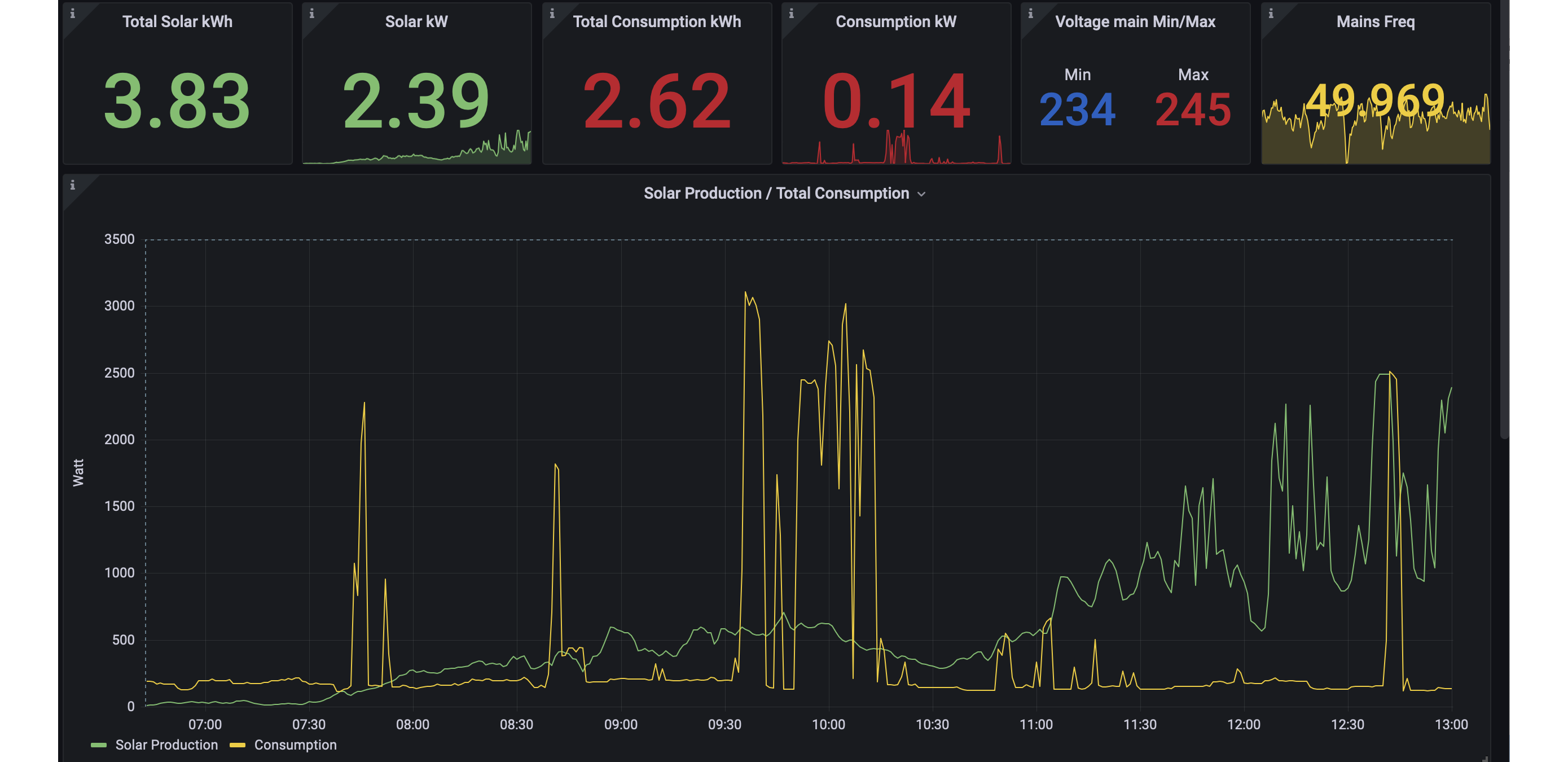
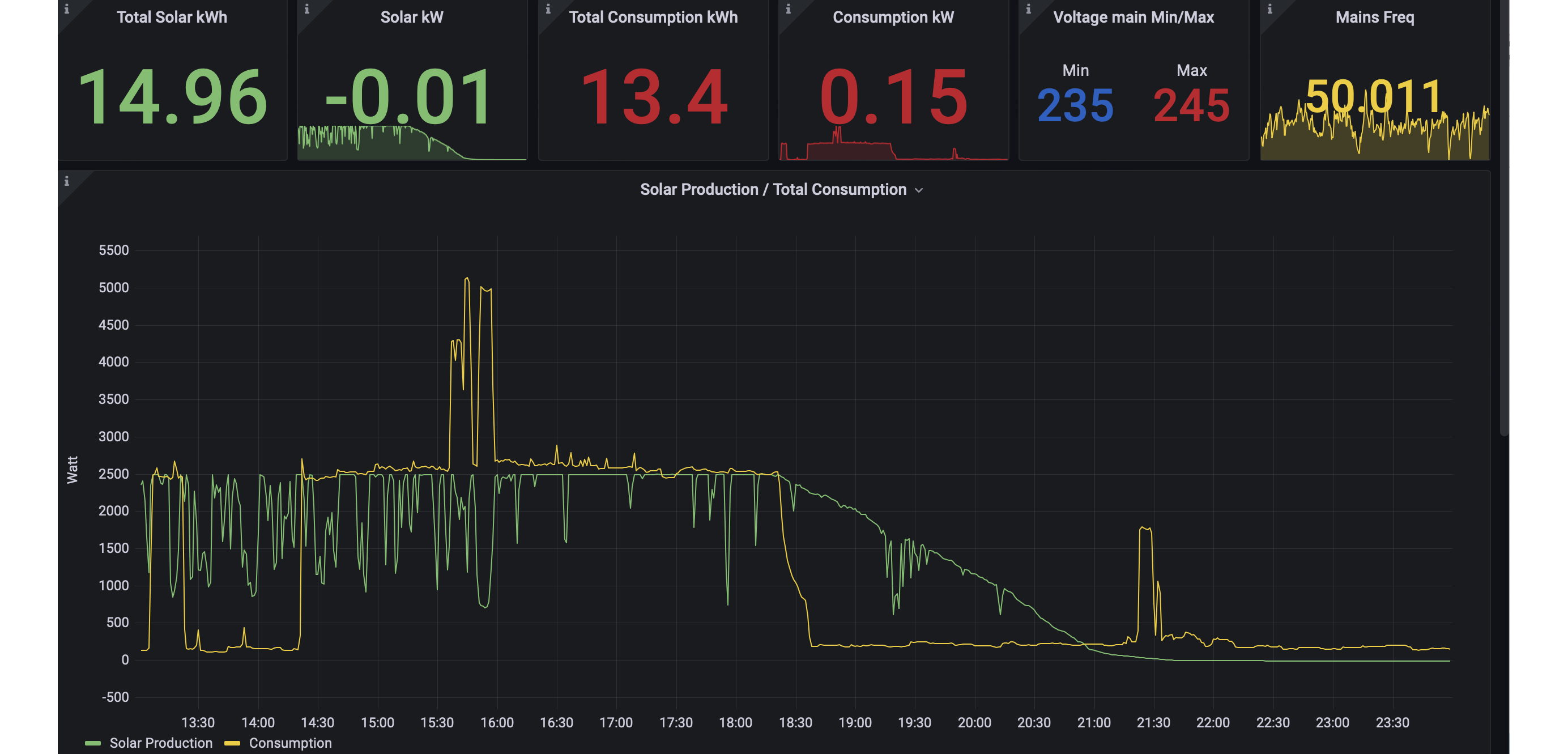
So, total production during ramp-up is 3.83 kWh whereas a total of 14.96 kWh is produced after 13:00.
These answers can be obtained in a matter of seconds whereas doing the same from Smappee would require one to download the raw data from the Smappee Cloud, import them in a spreadsheet to calculate the desired values. This would not only be a hassle, but it would also take way more time.
Let’s now look at the Power budget and Power import graphs. These represent the following data:
-
The Power budget is the difference between the generated power and the consumed power at a particular point in time. This value is non-zero if the former is larger than the latter, otherwise it is zero. So, this graph can tell us how much extra, non-utilised power the Solar panels generate over time. It can be considered a budget, hence the name Power budget. If we can store this energy, we can use it at a later time when we consume more than what is produced.
-
The Power import graphs is the sibling of the Power budget graph: it tells us how much more power would be needed to cover the total power usage in the house.
We can observe in the Solar Production / Total Consumption graph that there’s a steady consumption of about 2400 W between 14:20 and 18:20. This is actually the charging of the battery of a hybrid car. Even though quite a lot of energy is generated by the Solar panels, it is not sufficient to cover the full load of all consumers in the house. This can be seen from the Power budget and Power import graphs.
Unfortunately, these graphs are not that straightforward to generate, as the query language doesn’t have the required functions to do the calculation in a simple way. There’s no max (maximum) function that would allow us to calculate the Power budget values like this:
PB = max(solar_power - consumption_power, 0)There is an abs (absolute value) function though that allows us to obtain the desired value as follows:
PB = (solar_power - consumption_power + abs(solar_power - consumption_power))/2A bit contrived, but it does the job. Still, what we can’t compute in Grafana is the total Energy budget and the total Consumption Import values (both in kWh). This is due to the limitation of the Grafana sum function that doesn’t take computed values such as PB as argument. Still, it would be extremely useful to have these values. I plan to explore some alternative solutions for this after migrating to InfluxDB version 2.
Solar production numbers over a day
Let’s return to the Grafana dashboards. Here’s another question: imagine a day with no clouds in the sky. On such a day we would have a maximum amount of energy generation by the solar panel installation. What is the ratio between the energy generated during the ramp-up phase in the morning, the steady-state phase, and the ramp-down in the late afternoon? Let’s find such a day in the logged data and then get the answers in the same way as we did above.
Let’s zoom out a bit:
Well… it’s not been very sunny this spring, but it seems that April 19th may be a good candidate…
Ok, not perfect, but good enough as the total production that day was almost 20 kWh.
Repeating the process to select the appropriate numbers, we get:
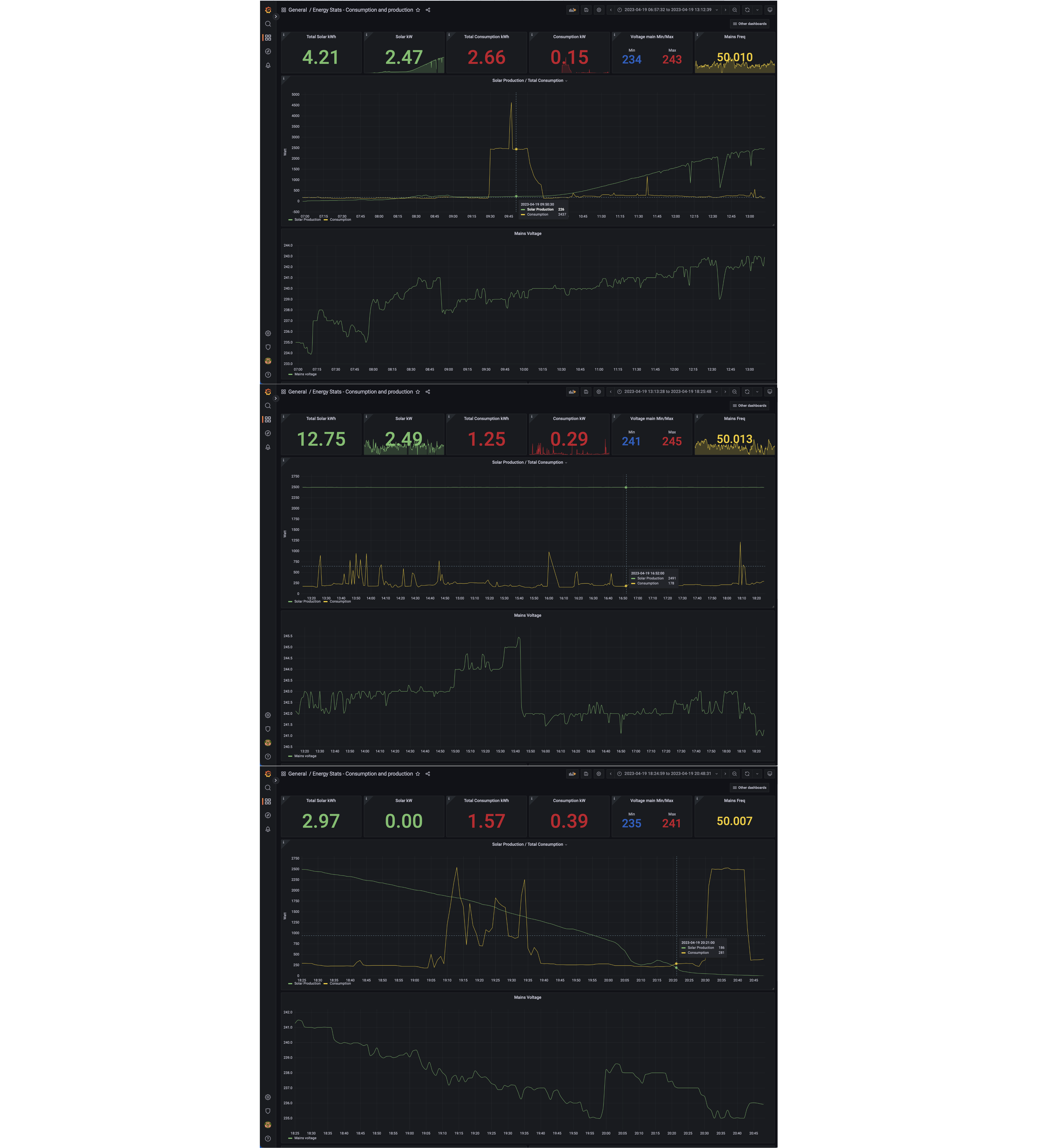
The amount of energy produced in each section of the production curve is 4.21 kWh, 12.75 kWh, and 2.97 kWh. When we express this as relative to total production number, we get the following ratios:
-
Ramp-up: 21.1%
-
Steady state: 64.0%
-
Ramp-down: 14.9%
The beautiful thing about this is that the exploration and calculation takes just a minute to complete.
The "Energy Stats - Consumer details" dashboard
This dashboard shows total energy consumption for all the measurements taken by the Smappee Infinity system (see the Smappee Infinity connection diagram).
It allows us to answer questions like:
-
What was the total energy consumption of:
-
the air-conditioning system last month?
-
the charging of the hybrid car’s battery last winter?
-
cooking fresh tomato sauce from the 15kg of tomatoes we bought the other day?
-
Ok, the last example is a bit far fetched but possible nevertheless and it’s a great topic to kickstart a conversation about energy (and cooking)!
The graphs can also tell us some interesting things like:
-
How does the power consumption of the air-conditioning system evolve between start-up and the reaching of a steady state?
-
How does the power used to charge the battery of an electrical bicycle evolve during a charging cycle?
For the question, we can have a look at this graph which display the airco power consumption on April 7th of this year:
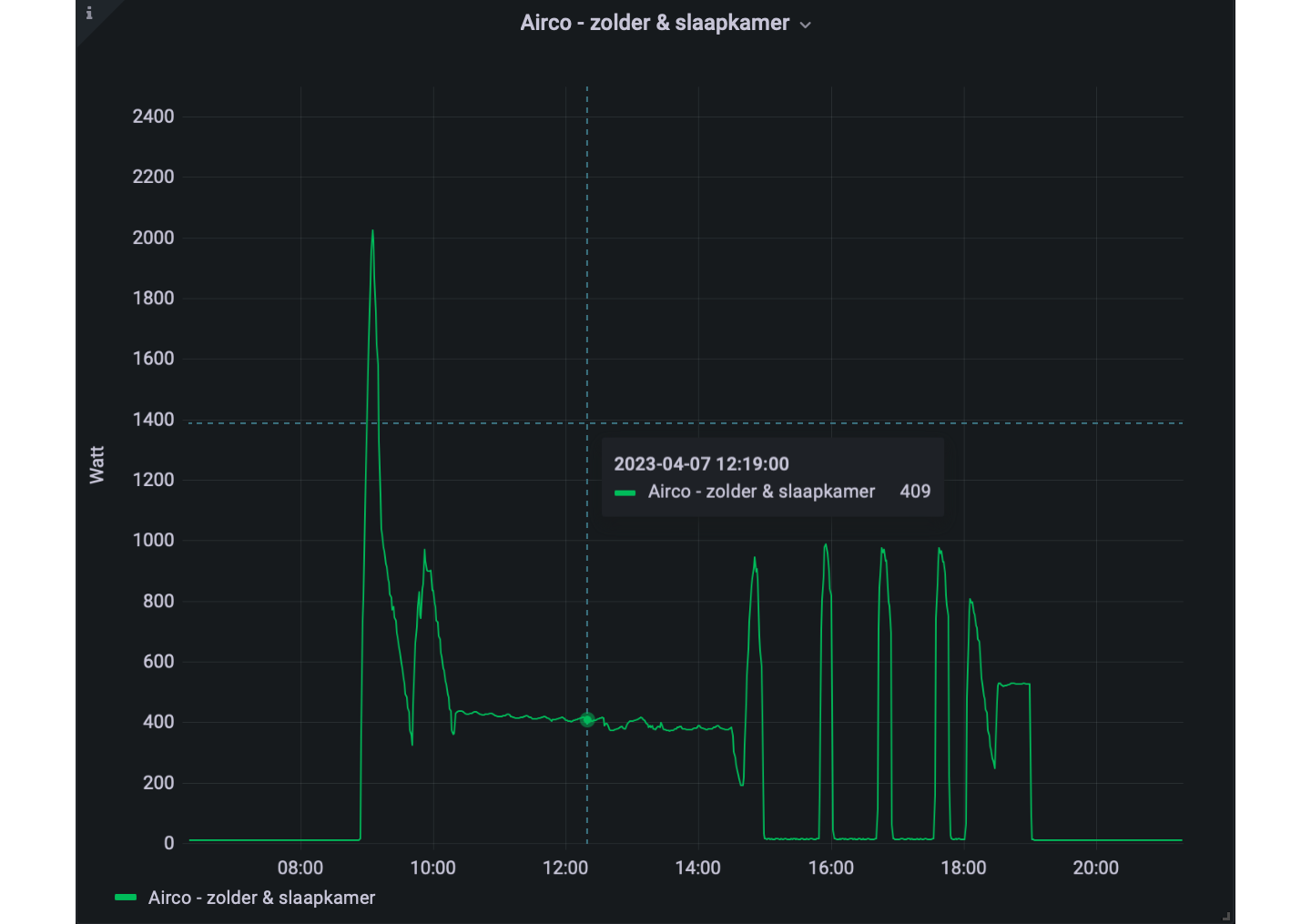
After an initial spike (with a peak of 2 kW) for about 20 minutes, the system evolves to a steady state where it consumes about 0.4 kW for about 4 hours, after which changes to a kind of on-off mode.
As for the second question, we can have a look at the following graph with data from May 15th:
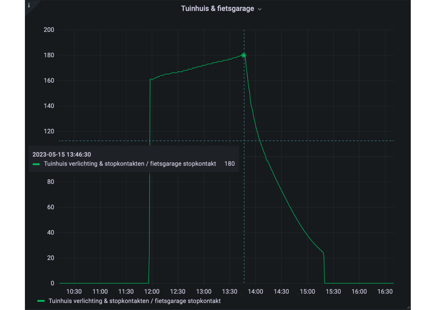
We see that the power at which the battery is charged rises from an initial value of ±160 W to ±180 W over a period of almost 2 hours. I think this is because it wasn’t very warm outside, the battery’s temperature rises during charging and the charging current is probably a function of that temperature, but that’s an unconfirmed and personal theory. After reaching the peak, the charging slows down and stops after another one and a half hour.
In conclusion, we can learn a lot about the different electrical consumers in the house and even learn a few special things about certain devices like the air-conditioning.
The Power Quality dashboard
This dashboard contains two graphs that display the following data for all channels on the Smappee Infinity:
-
Apparent and Real power
-
cos(φ)
We can have a look at the data for the garage when the hybrid car is being charged:
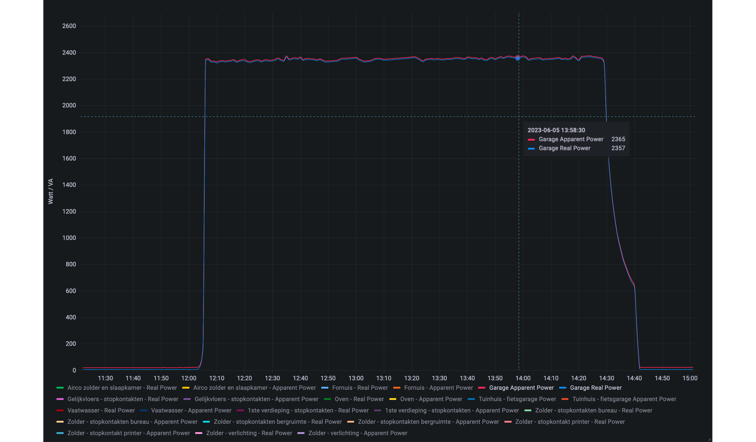
The apparent power and real power are 2365 VA and 2357 W respectively. This corresponds to a cos(φ) = 0.997 which is pretty much close to ideal. This is especially important as the power consumed during the charging is about 2.4 kW.
On the other hand, the charger of our electrical bicycle charger’s cos(φ) is only 0.69. So, when charging, the different powers are Preal = 180 W, Pa = 260 VA, and Preactive = 187 W. Even though it’s "only 187 W", when thousand or millions of devices with a low Power factor are online, the impact is significant.
Electrical Power Factor (also known as cos(φ))
The Power Factor is a measure of an electrical system’s energy utilisation efficiency. The power consumption can be decomposed in three parts:
-
Pa: Apparent power, which is the product of the measured voltage and current.
-
Preal: Effective or Real Power is the part that actually produces work in the broad sense of the word, it’s not the internal efficiency of the device itself. For example, an incandescent lightbulb consuming 100 W converts 98 W to heat and only 2 W to light. So, in this case, the Productive Power is 100 W (this is not to be confused with the efficiency of that bulb which is 2%).
-
Preactive: Reactive power (VAR - Volt-Ampère-Reactive) which is the part that doesn’t perform any work, but that still results in energy flowing between the electricity producer and consumer.
The relation between these components is the following:
-
P2a = P2real + P2reactive
-
Preal = Pa . cos(φ)
-
Preactive = Pa . sin(φ)
(If you’re interested about the theory around this topic, read this article about it.)
In electrical systems, cos(φ) is a value between 0 and 1. When the Reactive power is 0, cos(φ) is equal to 1 and Pa and Preal have equal values.
On the other extreme, Preactive is equal to Pa, and Preal and cos(φ) are both 0.
Both the real- and the reactive power components transfer energy between energy producer and consumer. The real power component corresponds to a unidirectional transfer of energy from producer to consumer. The reactive power component corresponds to energy being bounced back and forth between producer and consumer.
If we look at the bigger picture, both are transferred through the grid via high-voltage transmission lines, transformers, and local power distribution systems. During this transfer, losses occur amounting to 6% to 8% of the total energy produced.
Companies that produce and sell electricity want the reactive power to be 0 or as small as possible compared to the apparent power. This is because, in principle, the transmission losses generated by the reactive power aren’t billable to consumers. With the explosion of battery powered devices that use chargers such as mobile phones, laptop computers, electric bicycles, and electric cars, this poses a real challenge as these supplies may exhibit a poor cos(φ). Regulations are being put in place to force manufacturers to address this issue.
Future work
-
Upgrade of the production system without any loss of data
-
Upgrade Ubuntu 20.04 to Ubuntu 22.04
-
Upgrade InfluxDB v1 to InfluxDB v2
-
-
Add pricing and electricity cost data to the system
-
Add dashboards that display the price of electricity imported from (and exported to) the grid over a specified period and for specific consumers
-
Add dashboards that display cost data such as day-ahead prices and that calculate the actual cost of power consumption (or the money received as a result of injecting electricity into the grid)
-
-
Actively control electricity consumption to:
-
Reduce peak consumption
-
Drive down the electricity bill by shifting consumption to moments where the prices are lower. Candidate consumers are electrical water boilers and electric cars
-
Glossary
| Term | Definition |
|---|---|
DC |
Direct Current. A DC system is one where voltages and currents always have the same polarity in function of time. Note the loose utilisation of the term current: in general the term direct applies to both voltages and currents in an electrical system. |
AC |
Alternating Current. Most AC systems have voltages and currents that change polarity periodically. The actual waveform can be sinusoidal, but doesn’t have to be. With the advent of [power] electronics, currents may deviate a lot from the ideal sine wave form. In general, such deviations are undesirable as these may cause electromagnetic interference (EMI) issues. |
W |
Watt, abbreviated as W is the metric unit for power. From a mechanical point of view, it is equal to 1 Joule/second where 1 Joule is the amount of energy used when exerting a force of 1 Newton over a distance of 1 meter. In electrical terms, a 1 Volt battery that is discharging a 1 Ampère current to a consumer, generates a power of 1 Watt. |
VA |
Volt-Ampère, a unit of so-called apparent power, mostly applicable to AC systems. The apparent power is calculated by multiplying the voltage measured over a consumer by the measured current flowing through that consumer. Depending on the type of consumer, the current and the voltage may be phase-shifted. This leads to the appearance of a real- (or effective) and a reactive power component, expressed respectively in Watt and VAR. |
VAR |
Volt-Ampère-Reactive, a unit of so-called reactive power. It’s just a unit of power, but as it is used to characterise the reactive power component in an AC system, it’s not expressed in Watts. |
RMS |
Root-Mean-Square. It is applicable to systems with periodic wave forms. A typical example is the use in AC systems. For pure sinusoidal wave forms, the RMS value is equal to the amplitude of the sine wave divided by √2. As a concrete example, when we talk about a 240V AC system, it means that the voltage sine wave has an RMS value equal to 240V. The amplitude (or peak) value is 240V * √2 = 339V. |
cos(φ) |
cosine of φ, where φ is the phase shift between waveforms of voltage and current. Also known as Power factor. Ideally, electrical consumers should have a cos(φ) equal to 1. Deviations from this ideal lead to non-zero reactive current- and power components which in turn lead to transmission losses. Note that cos(φ) can be generalised to non-sinusoidal waveforms. |